This reading is part of our introductory options course. Please check out the full overview of lessons here.

1. What is the Value of an Option?

The value of a forward or futures contract is zero at the start of the contract, but it changes as prices or rates change. As prices or interest rates change, a contract that has positive value to one party and negative value to the other can reverse and have negative value to the former and positive value to the latter. The forward or futures price is the price at which the parties agree to buy and sell the underlying at a future date.

With options, these concepts are different. An option has a positive value at the start. The buyer must pay money and the seller receives money to initiate the contract. Prior to expiration, the option always has positive value to the buyer and negative value to the seller. Conversely, in a forward or futures contract, the two parties agree on the fixed price the buyer will pay the seller. This fixed price is set such that the buyer and seller do not exchange any money. The corresponding fixed price at which a call holder can buy the underlying or a put holder can sell the underlying is the exercise price. It is also negotiated between the buyer and the seller, but the buyer still pays the seller money up front in the form of an option premium or price.¹

Thus, what we call the forward or futures price corresponds more to the exercise price of an option. 

Before we begin, it’s vital to highlight that we assume that all market players are rational, in the sense that they don’t waste money and take advantage of arbitrage opportunities. As a result, we assume that markets are sufficiently efficient to prevent arbitrage.

Let us start by developing the notation. Note that time 0 is today and time T is the expiration.

S₀, S_T = price of the underlying asset at time 0 (today) and time T (expiration)

X = exercise price

r = risk-free rate

T = time to expiration, equal to number of days to expiration divided by 365

c₀, c_T = price of European call today and at expiration

C₀, C_T = price of American call today and at expiration

p₀, Cp_T = price of European put today and at expiration

P₀, P_T = price of American put today and at expiration

On occasion, we will introduce some variations of the above as well as some new notation. For example, we start off assuming that the underlying has no cash flows.

2.     Payoff Values

The easiest time to determine an option’s value is at expiration. At that point, there is no future. Only the present matters. The value of an option at expiration is known as its payoff. 

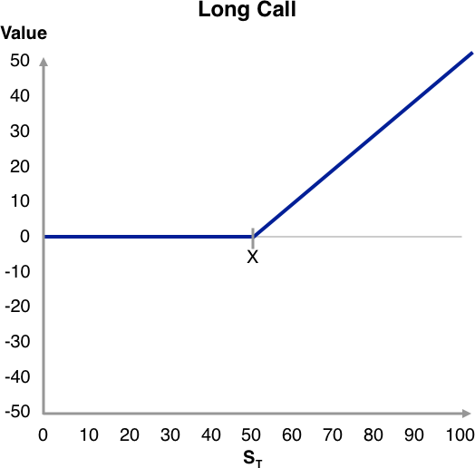
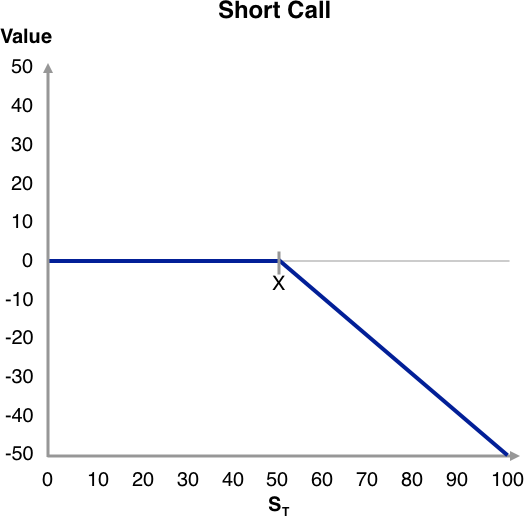
At expiration, a call option is worth either zero or the difference between the underlying price and the exercise price, whichever is greater:

c_T = Max (0, S_T – X)

C_T = Max (0, S_T – X)

It is worth noting that at expiration, a European option and an American option have the same payoff because they are equivalent instruments at this point.

Max(0, S_T – X) denotes the greater of zero or S_T – X. Assume the underlying price is greater than the exercise price, S_T > X. In this case, the option expires in-the-money and the option is worth S_T – X. Assume that at the time of expiration, it is possible to buy the option for less than S_{T –} X. Then one could buy the option, immediately exercise it, and immediately sell the underlying. Doing so would cost c_T (or C_T) for the option and X to buy the underlying but would bring in S_T for the sale of the underlying. If c_T (or C_T) < S_T – X, this transaction would net an immediate risk-free profit. The collective actions of all investors doing this would force the option price up to S_T – X. The price could not go higher than S_T – X, because all that the option holder would end up with an instant later when the option expires is S_T – X. If S_T < X meaning that the call is expiring out-of-the-money, the formula says the option should be worth zero. It cannot sell for less than zero because that would mean that the option seller would have to pay the option buyer. A buyer would not pay more than zero, because the option will expire an instant later with no value.

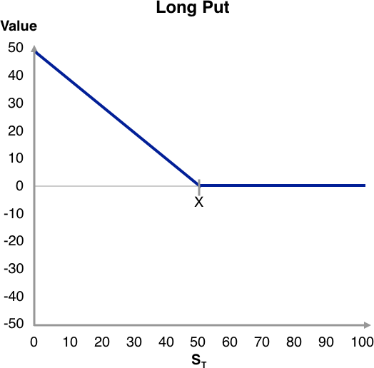
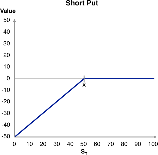
At expiration, a put option is worth either zero or the difference between the exercise price and the underlying price, whichever is greater:

p_T = Max (0, X – S_T)

P_T = Max (0, X – S_T)

Assume S_T < X, indicating that the put is expiring in-the-money. The put is selling for less than X – S_T at expiration. The investor then purchases the put for p_T (or P_T) and the underlying for S_T and exercises the put and receives X. If p_T (or P_T) < X – S_T, this transaction will result in an immediate risk-free profit. The combined actions of participants doing this will force the put price up to X – S_T. It cannot go any higher, because the put buyer will end up an instant later with only X – S_T and would not pay more than this. If S_T > X, the put is worth nothing because it will expire out-of-the-money. It cannot be less than zero because the option seller must pay the option buyer. It cannot be worth more than zero because the buyer would not pay for a position that would be worth nothing an instant later.

These important findings are summarized along with an example in the Exhibit below. The payoff diagrams for the short positions are also shown and are obtained as the negative of the long positions. For the special case of S_T = X, meaning that both call and put are expiring at-the-money, we can effectively treat the option as out-of-the-money because it is worth zero at expiration.

The value Max (0, S_T – X) for calls or Max (0, X – S_T) for puts is also called the option’s intrinsic value or exercise value. We shall use the former terminology. Intrinsic value is what the option is worth to exercise it based on current conditions. We have only discussed the option at expiration in this section. An option will typically sell for more than its intrinsic value prior to expiration.² The difference between the option’s market price and intrinsic value is known as its time value or speculative value. We shall use the former terminology. The time value reflects the potential for the option’s intrinsic value at expiration to be greater than its current intrinsic value. Of course, at expiration, the time value is zero.

Exhibit: Option Values and Payoff Profiles at Expiration (Payoffs)

Option	Value	Example (X = 50; ST = 55)	Example (X = 50; ST = 45)
European call	cT = Max (0, ST – X)	cT = Max (0, 55 – 50) = 5	cT = Max (0, 45 – 50) = 0
American call	CT = Max (0, ST – X)	CT = Max (0, 55 – 50) = 5	CT = Max (0, 45 – 50) = 0
European put	pT = Max (0, X – ST)	pT = Max (0, 50 – 55) = 0	pT = Max (0, 50 – 45) = 5
American put	PT = Max (0, X – ST)	PT = Max (0, 50 – 55) = 0	pT = Max (0, 50 – 45) = 5

• 

• 

• 

• 

Everyone agrees on the intrinsic value of the option; after all, it is based on the current stock price and exercise price. We have more difficulty estimating the time value. So, keeping in mind that Option price = intrinsic value + time value, let us proceed and try to determine the value of an option today, prior to expiration.

3.     Boundary Conditions

We begin by looking at some simple results that establish minimum and maximum values for options before they expire.

3.1      Minimum and Maximum Values

The first and perhaps most obvious result is one we have already discussed: The minimum value of any option is zero. We state this formally as:

c₀ > 0, C₀ > 0

p₀ > 0, P₀ > 0

No option can sell for less than zero, because the seller would then have to pay the buyer.

Now consider the maximum value of an option. It varies depending on whether the option is a call or a put, as well as whether it is European or American. The current value of the underlying is the maximum value of a call:

c₀ < S₀, C₀ < S₀

A call is a method of buying the underlying. It would not make sense to pay more for the right to buy the underlying than the value of the underlying itself. 

When it comes to puts, whether they are European or American makes a difference. Consider the best possible outcome for the put holder when determining the maximum value for puts. The best-case scenario is for the underlying to reach a value of zero. The put holder can then sell a worthless asset for X. The holder of an American put could sell it immediately and profit by X. For a European put, the holder must wait until expiration; thus, we must discount X from the expiration date to the present. As a result, the present value of the exercise price is the maximum value of a European put. For an American put the exercise price is the maximum value.

p₀ < X/(1 + r)^T, P₀ < S₀

where r is the risk-free interest rate and T is the time to expiration. These results for the maximums and minimums for calls and puts are summarized in the Exhibit below, which also includes a numerical example.

Exhibit: Minimum and Maximum Values of Options

Option	Minimum Value	Maximum Value	Example (S0 = 55, X = 50, r = 3%, T = ½ year)
European call	c0 > 0	c0 < S0	0 < c0 < 55
American call	C0 > 0	C0 < S0	0 < C0 < 55
European put	p0 > 0	p0 < X/(1 + r)T	0 < p0 < 49.27 [49.27 = 50 / (1.03)0.5]
American put	P0 > 0	P0 < S0	0 < P0 < 50

3.2      Lower Bounds

The results established in the preceding section do not impose many constraints on the option price. They tell us that the price is between zero and the maximum, which is either the underlying price, the exercise price, or the present value of the exercise price—a fairly broad range of possibilities. Fortunately, we can narrow the range slightly on the low end as we can set a lower bound on the option price.

For American options, which are exercisable immediately, we can state that the lower bound of an American option price is its current intrinsic value (in fact, we will shortly demonstrate that we can override one of these results with a lower bound that is higher and thus a better lower bound):

C₀ > Max(0, S₀ – X)

P₀ > Max(0, X – S₀)

The reason why these results hold today is the same reason why they must hold at expiration. If the option is in the money and selling for less than its intrinsic value, it can be purchased and exercised immediately for a risk-free profit. The collective actions of market participants will force the American option price to at least equal the intrinsic value.

Unfortunately, such a statement cannot be made about European options, but we can show that the lower bound is either zero or the current underlying price minus the present value of the exercise price, whichever is greater. They cannot be exercised early, so market participants cannot exercise an option that is selling for too little in relation to its intrinsic value. Fortunately, there is a way to set a lower bound on European options. We can combine options with risk-free bonds and the underlying to obtain a lower bound on the option price.

To begin, we must be able to purchase and sell a risk-free bond with a face value equal to the exercise price and a current value equal to the present value of the exercise price. This procedure is straightforward, but it may not be obvious. If the exercise price is X (say, 100), we purchase a bond with a face value of X (100) that matures on the option expiration date. The current value of that bond is the present value of X, which is X/(1 + r)^T . So we buy the bond today for X/(1 + r)^T and hold it until it matures on the option expiration day, at which time it will pay off X. We assume that we can buy or sell (issue) this type of bond. It should be noted that this transaction entails borrowing or lending an amount equal to the present value of the exercise price, with repayment of the full exercise price.

The Exhibit below depicts the construction of a unique combination of instruments. We purchase the European call and the risk-free bond and sell the underlying asset short. Remember that short selling entails borrowing an asset and selling it. We will purchase the asset at the end of the term. In order to illustrate the logic behind the lower bound for a European call in the simplest way, we assume that we can sell short without any restrictions.

In the Exhibit below the two right-hand columns contain the value of each instrument when the option expires. The rightmost column is the case of the call expiring in-the-money, in which case it is worth S_T – X. In the other column, the out-of-the-money case, the call is worth zero. The underlying is worth –S_T (the negative of its current value) in either case, reflecting the fact that we buy it back to cover the short position. The bond is worth X in both cases. When the option expires out-of-the-money, the sum of all positions is positive; when the option expires in-the-money, the sum of all positions is zero. As a result, in no case does this instrument combination have a negative value. That means we’ll never have to pay out any money when the contract expires. We are guaranteed at least no loss and possibly a profit at expiration.

Exhibit: A Lower Bound Combination for European Calls

Transaction	Current Value	Value at Expiration (ST < X)	Value at Expiration (ST > X)
Buy call	c0	0	ST – X
Sell short underlying	-S0	-ST	-ST
Buy bond	X/(1 + r)T	X	X
Total	c0 – S0 + X/(1 + r)T	X – ST > 0	0

If there is a possibility of a positive outcome from the combination, and we know we will never have to pay anything out from holding the combination of instruments, the cost of that combination must be positive—it must cost us something to enter the position. We cannot accept money in order to enter the position. In that case, we would receive money up front and never have to pay it back.

The cost of entering the position is shown in the second column, labelled the “Current Value”. Because that value must be positive, we therefore require that c₀ – S₀ + X/(1 + r)^T > 0. Rearranging this equation, we obtain c₀ > S₀ – X/(1 + r)^T.  We now have a statement about the minimum value of the option, which can serve as a lower bound. This result is solid, because if the call is selling for less than S₀ – X/(1 + r)^T, an investor can buy the call, sell short the underlying, and buy the bond. This would bring in money up front, and as shown in the Exhibit, an investor would not have to pay out any money at expiration, and might even get a little more. Because other investors would do the same, the call price would be forced up until it is at least S₀ – X/(1 + r)^T.

But we can improve on this result. Suppose S₀ – X/(1 + r)^T is negative. Then we are stating that the call price is greater than a negative number. We already know, however, that the call price cannot be negative. As a result, we can now state that:

c₀ > Max(0, S₀ – X/(1 + r)^T)

In other words, the lower bound on a European call price is either zero or the underlying price minus the present value of the exercise price, whichever is greater. Notice how this lower bound differs from the lower bound for the American call, Max (0, S₀ – X). We must wait to pay the exercise price and obtain the underlying for the European call. As a result, the expression includes both the current underlying value (the present value of its future value) and the present value of the exercise price. Because we do not have to wait until expiration for the American call, the expression reflects the possibility of receiving the underlying price minus the exercise price right away. 

To illustrate the lower bound, let X = 50, r = 3%, and T = 0.5. If the current underlying price is 45, then the lower bound for the European call is:

Max(0, 45 – 50 / (1.03)^0.5) = Max (0, 45 – 49.27) = Max(0, –4.27) = 0

All this calculation tells us is that the call must be worth no less than zero, which we already knew. If the current underlying price is 55, however, the lower bound for the European call is:

Max (0, 55 – 49.27) = Max (0, 5.63) = 5.63

This tells us that the call must be worth no less than 5.63. In this same application of the present value of the exercise price, we can see that the lower bound on European puts differs from the lower bound on American puts.

Exhibit: A Lower Bound Combination for European Puts

Transaction	Current Value	Value at Expiration (ST < X)	Value at Expiration (ST > X)
Buy call	p0	X – ST	0
Sell short underlying	S0	ST	ST
Buy bond	–X/(1 + r)T	–X	–X
Total	p0 + S0 – X/(1 + r)T	0	ST – X > 0

The example above shows how to build a portfolio of European puts in a similar manner. However, in this case, we purchase the put and the underlying and borrow by issuing the zero-coupon bond. Each instrument’s payoff is indicated in the two rightmost columns. It is worth noting that the total payoff is never less than zero. Consequently, the initial value of the combination must not be less than zero. Therefore, p₀ + S₀ – X/(1 + r)^T > 0. Isolating the put price gives us p₀ > X/(1 + r)^T – S₀. But suppose that X/(1 + r)^T – S₀ is negative. Then, the put price must be greater than a negative number. We know that the put price must be no less than zero. So, we can now formally say that:

p₀ > Max(0, X/(1 + r)^T – S₀)

In other words, the lower bound of a European put is the greater of either zero or the present value of the exercise price minus the underlying price. For the American put, recall that the expression was Max(0, X – S₀). So, for the European put, we adjust this value to the present value of the exercise price. The present value of the asset price is already adjusted to S₀.

Using the same example we did for calls, let X = 50, r = 3%, and T = 0.5. If the current underlying price is 45, then the lower bound for the European put is:

Max (0, 50 / (1.03)^0.5 – 45) = Max (0, 49.27 – 45) = Max (0, 4.27) = 4.27

If the current underlying price is 55, however, the lower bound is:

Max (0, 49.27 – 55) =  Max (0, –5.63) = 0

At this point let us reconsider what we have established. The lower bound for a European call is Max(0, S₀ – X/(1 + r)^T). We also observed that an American call must be worth at least Max(0, S₀ – X). Except upon expiry, the European lower bound is greater than the American call’s minimum value. However, we couldn’t expect an American call to be valued less than a European call. As a result, the lower bound of the European call also applies to American calls. As a result, we can conclude:

c₀ > Max(0, S₀ – X/(1 + r)^T)

C₀ > Max(0, S₀ – X/(1 + r)^T)

For European puts, the lower bound is Max(0, X/(1 + r)^T – S₀). For American puts, the minimum price is Max(0, X – S₀). The European lower bound is lower than the minimum price of the American put, so the American put’s lower bound is not changed to the European lower bound, the way we did for calls. Hence,

p₀ > Max(0, X/(1 + r)^T – S₀)

P₀ > Max(0, X – S₀)

These results tell us the lowest possible price for European and American options.

Recall that we previously referred to an option price as having an intrinsic value and a time value. For American options, the intrinsic value is the value if exercised, Max(0, S₀ – X). for calls and Max(0, X – S₀). for puts. The time value is the rest of the option price. For European options, the concept of time value is somewhat hazy because it first necessitates the understanding of intrinsic worth. Because a European option cannot be exercised until it expires, all of its value is essentially time value. The idea of intrinsic value and its complement, time value, are thus inadequate for European options, despite the fact that the ideas are often applied to European options. Fortunately, understanding European options does not necessitate distinguishing between intrinsic and time value. We’ll group them together because they make up the option price.

4.     The Effect of Difference in Exercise Price

Now consider two options on the same underlying with the same expiration date but different exercise prices. In general, the greater the exercise price, the less valuable a call is and the more valuable a put is. To see this, let the two exercise prices be X₁ and X₂, with X₁ being the smaller. Let c₀(X₁) be the price of a European call with exercise price X₁ and c₀(X₂) be the price of a European call with exercise price X₂. We refer to these as the X₁ call and the X₂ call. In the below Exhibit, we construct a combination in which we buy the X₁ call and sell the X₂ call.³

Exhibit: Portfolio Combination for European Calls Illustrating the Effect of Differences in Exercise Prices

Transaction	Current Value	Value at Expiration (ST < X1)	Value at Expiration (X1 < ST < X2)	Value at Expiration (ST > X2)
Buy call (X = X1)	c0(X1)	0	ST – X1	ST – X1
Sell call (X = X2)	– c0(X2)	0	0	– (ST – X2)
Total	c0(X1) – c0(X2)	0	ST – X1 > 0	X2 – X1 > 0

Note first that the three outcomes are all non-negative. This fact demonstrates that the current value of the combination, c₀(X₁) – c₀(X₂) has to be non-negative. We have to pay out at least as much for the X₁ call as we take in for the X₂ call; otherwise, we would get money up front, have the possibility of a positive value at expiration, and never have to pay any money out. Thus, because c₀(X₁) – c₀(X₂) > 0, we restate this result as:

c₀(X₁) > c₀(X₂)

This phrase means that a call option with a greater exercise price cannot have a higher value than one with a lower exercise price. Because the option with the higher exercise price has a larger barrier to overcome, the buyer is unwilling to spend as much for it. Although we established this finding with European calls, it also applies to American calls. Thus:⁴

C₀(X₁) > C₀(X₂)

In the Exhibit below we construct a similar portfolio for puts, except that we buy the X₂ put (the one with the higher exercise price) and sell the X₁ put (the one with the lower exercise price).

Exhibit: Portfolio Combination for European Puts Illustrating the Effect of Differences in Exercise Prices

Transaction	Current Value	Value at Expiration (ST < X1)	Value at Expiration (X1 < ST < X2)	Value at Expiration (ST > X2)
Buy put (X = X2)	p0(X2)	X2 – ST	X2 – ST	0
Sell put (X = X1)	– p0(X1)	– (X1 – ST)	0	0
Total	p0(X2) – p0(X1)	X2 – X1 > 0	X2 – ST > 0	0

Observe that the value of this combination is never negative at expiration; therefore, it must be non-negative today. Hence, p₀(X₂) – p₀(X₁) > 0. We restate this result as:

p₀(X₂) > p₀(X₁)

As a result, the value of a European put with a greater exercise price must be at least equal to that of a European put with a lower exercise price. These findings also apply to American puts. As a result:

P₀(X₂) > P₀(X₁)

Even though it is technically possible for calls and puts with different exercise prices to have the same price, generally we can say that the higher the exercise price, the lower the price of a call and the higher the price of a put.

5.     The Effect of a Difference in Time to Expiration

Option pricing are also influenced by the option’s expiration date. Intuitively, the longer the period to expiry, the more valuable the option. A longer-term option gives the underlying more time to make a beneficial move. Furthermore, if the option is in-the-money at the conclusion of a specific time period, it has a greater probability of moving even more in-the-money over a longer time period. If the additional time increases the likelihood of moving out-of-the-money or farther out-of-the-money, the limiting of losses to the amount of the option premium implies that the disadvantage of the longer period is not larger. A longer time to expiry is usually advantageous for an option. Longer-term American and European calls, as well as longer-term American puts, will be worth no less than their shorter-term equivalents.

First let us consider each of the four types of options: European calls, American calls, European puts, and American puts. We shall introduce options otherwise identical except that one has a longer time to expiration than the other. The one expiring earlier has an expiration of T₁ and the one expiring later has an expiration of T₂. The prices of the options are c₀(T₁) and c₀(T₂) for the European calls, C₀(T₁) and C₀(T₂) for the American calls, p₀(T₁) and p₀(T₂) for the European puts, and P₀(T₁) and P₀(T₂) for the American puts.

When the shorter-term call expires, the European call is worth Max(0, S_T1 – X), but we have already shown that the longer-term European call is worth at least Max(0, S_T1 – X/(1 +r)^{(T2 – T1)}), which is at least as great as this amount. As a result, the longer-term European call is at least as valuable as the shorter-term European call. These results are not altered if the call is American. When the shorter-term American call expires, it is worth Max(0, S_T1 – X). The longer-term American call must be worth at least the value of the European call, so it is worth at least Max(0, S – X/(1 +r)^{(T2 – T1)}). As a result, when the shorter-term call expires, the longer-term call, whether European or American, is no less valuable than the shorter-term call. Because this assertion is always true, the longer-term call, whether European or American, is always worth no less than the shorter-term call at any point before expiry. Thus:

c₀(T₂) > c₀(T₁)

C₀(T₂) > C₀(T₁)

It is important to note that these assertions do not imply that the longer-term call is necessarily worth more; rather, they imply that the longer-term call cannot be worth less. Except in the rare scenario where both calls are so far out-of-the-money or in-the-money that the additional time to expiration is meaningless, the longer-term call will be worth more.

For European puts, we have a slight problem. In the case of calls, the longer duration allows for more time for a beneficial move in the underlying to occur. This is also true for puts, although there is one downside to waiting the extra time. When a put option is exercised, the holder is paid. The loss of interest on money is a downside of the extra time. There is no loss of interest for calls. In reality, by paying out the exercise price later, a call holder gains additional interest on the money. Therefore, it is not always true that additional time is beneficial to the holder of a European put. It is true, however, that the additional time is beneficial to the holder of an American put. An American put can always be exercised; there is no penalty for waiting. Thus, we have:

p₀(T₂) can be either greater or less than p₀(T₁)

P₀(T₂) > P₀(T₁)

As a result, for European puts, either the longer-term or shorter-term option may be more valuable. When volatility is high and interest rates are low, the longer-term European put will be more valuable. We might observe an exception to this rule for European puts, but these are all American options.

6.     Put-Call Parity

So far we have been working with puts and calls independently. To see how their prices must be consistent with each other and to explore common option strategies, let us combine puts and calls with each other or with a risk-free bond. We shall put together some combinations that produce equivalent results.

6.1      Fiduciary Calls and Protective Puts

First, we will look at a fiduciary cal option strategy. It is made up of a European call and a risk-free bond, similar to the ones we’ve been using, that matures on the option expiry day and has a face value equal to the call’s exercise price. The payoffs upon the expiration of the fiduciary call are shown in the upper portion of the table in the following Exhibit. We see that if the price of the underlying is below X at expiration, the call expires worthless and the bond is worth X. If the price of the underlying is above X at expiration, the call expires and is worth S_T (the underlying price) – X. So at expiration, the fiduciary call will end up worth X or ST, whichever is greater. This type of combination is called a fiduciary call because it allows protection against downside losses and is thus faithful to the notion of preserving capital.

Now we construct a strategy known as a protective put, which consists of a European put and the underlying asset. If the price of the underlying is below X at expiration, the put expires and is worth X – S_T and the underlying is worth S_T. If the price of the underlying is above X at expiration, the put expires with no value and the underlying is worth S_T. Consequently, at expiration, the protective put is worth X or S_T, whichever is greater. The lower part of the table in below Exhibit shows the payoffs at expiration of the protective put.

Exhibit: Portfolio Combination for Equivalent Packages of Puts and Calls

Transaction	Current Value	Value at Expiration (ST < X)	Value at Expiration (ST > X)
Fiduciary Call:
Buy call	c0	0	ST – X
But Bond	X/(1 + r)T	X	X
Total	c0 + X/(1 + r)T	X	ST
Protective Put:
Buy put	p0	X – ST	0
Buy underlying asset	S0	ST	ST
Total	p0 + S0	X	ST

As the fiduciary call and protective put end up with the same value, they are identical combinations. To avoid arbitrage, their values today must be the same. The value of the fiduciary call is the cost of the call, c₀, and the cost of the bond, X/(1 + r)^T. The value of the protective put is the cost of the put, p₀, and the cost of the underlying, S₀. Thus:

c₀ + X/(1 + r)^T = p₀ + S₀

This equation is called put-call parity and is one of the most important results in options. It does not state that puts and calls are equivalent, but it does show an equivalence (parity) of a call/bond portfolio and a put/underlying portfolio.

Put-call parity can be written in a number of other ways. By rearranging the four terms to isolate one term, we can obtain some interesting and important results. For example:

c₀ = p₀ + S₀ – X/(1 + r)^T

This means that a call is equivalent to a long position in the put, a long position in the asset, and a short position in the risk-free bond. The short bond position simply means to borrow by issuing the bond, rather than lend by buying the bond as we did in the fiduciary call portfolio. We can tell from the sign whether we should go long or short. Positive signs mean to go long; negative signs mean to go short.

6.2      Synthetics

Because the right-hand side of the above equation is equivalent to a call, we often refer to it as a synthetic call. To see that the synthetic call is equivalent to the actual call, please refer to the below exhibit.

Exhibit: Call and Synthetic Call

Transaction	Current Value	Value at Expiration (ST < X)	Value at Expiration (ST > X)
Call:
Buy call	c0	0	ST – X
Synthetic Call:
Buy put	p0	X – ST	0
Buy underlying asset	S0	ST	ST
Issue bond	–X/(1 + r)T	–X	–X
Total	p0 + S0 – X/(1 + r)T	0	ST – X

The call yields the underlying’s value less the exercise price or zero, whichever is larger. The synthetic call does the same thing, but in a different manner. When the call expires in-the-money, the synthetic call yields the underlying value less the bond payout, which is X. When the call expires out-of-the-money, the put covers the loss on the underlying, and the put’s exercise price corresponds to the amount of money required to pay off the bond.

Similarly, we can isolate the put as follows:

p₀ = c₀ – S₀ + X/(1 + r)^T

which says that a put is equivalent to a long call, a short position in the underlying, and a long position in the bond. Because the left-hand side is a put, it follows that the right-hand side is a synthetic put. The equivalence of the put and synthetic put is shown in below Exhibit.

Exhibit: Put and Synthetic Put

Transaction	Current Value	Value at Expiration (ST < X)	Value at Expiration (ST > X)
Put:
Buy put	p0	X – ST	0
Synthetic Put:
Buy call	c0	0	ST – X
Short underlying asset	–S0	–ST	–ST
Buy bond	X/(1 + r)T	X	X
Total	c0 – S0 + X/(1 + r)T	X – ST	0

As you may expect, there are several different combinations that may be created. The Exhibit below depicts some of the more important combinations.

Exhibit: Alternative Equivalent Combinations of Calls, Puts, the Underlying, and Risk-Free Bonds

Strategy	Consisting Of	Worth	Equates To	Strategy	Consisting Of	Worth
Fiduciary Call	Long call + Long bond	c0 + X/(1 + r)T	=	Protective put	Long put + Long underlying	p0 + S0
Long call	Long call	c0	=	Synthetic call	Long put + Long underlying + Short bond	p0 + S0 – X/(1 + r)T
Long put	Long put	p0	=	Synthetic put	Long call + Short underlying + Long bond	c0 – S0 + X/(1 + r)T
Long underlying	Long underlying	S0	=	Synthetic underlying	Long call + Long bond + Short put	c0 + X/(1 + r)T – p0
Long bond	Long bond	X/(1 + r)T	=	Synthetic bond	Long put + Long underlying + Short call	p0 + S0 – c0

There are two main reasons why understanding synthetic positions in option pricing is crucial. Because synthetic positions yield the same effects as options and have established prices, they allow us to price options. Synthetic positions also demonstrate how to profit from option mispricing in relation to their underlying assets. It’s worth noting that we may synthetically create not only a call or a put, but also the underlying or the bond. As difficult as it may appear to execute this, it is actually fairly simple. First, we learn that a fiduciary call is a call plus a risk-free bond maturing on the option expiration day with a face value equal to the exercise price of the option. Then we learn that a protective put is the underlying plus a put. Then we learn the basic put-call parity equation: A fiduciary call is equivalent to a protective put:

c₀ + X/(1 + r)^T = p₀ + S₀

Learn the put-call parity equation this way, because it is the easiest form to remember and has no minus signs.

6.3      An Arbitrage Opportunity

In this section we examine the arbitrage strategies that will push prices to put-call parity. Suppose that in the market, prices do not conform to put-call parity. This is a situation in which price does not equal value. Recalling our basic equation, c₀ + X/(1 + r)^T = p₀ + S₀, we can insert values into the equation and see if the equality holds. If it does not, then obviously one side is greater than the other. We can view one side as overpriced and the other as underpriced, which suggests an arbitrage opportunity. To exploit this mispricing, we buy the underpriced combination and sell the overpriced combination.

Consider the following example involving call options with an exercise price of 50 expiring in half a year (T = 0.5). The risk-free rate is 3 percent. The call is priced at 4.50, and the put is priced at 5.25. The underlying price is 49.

The left-hand side of the basic put-call parity equation is c₀ + X/(1 + r)^T = 4.50 + 50 / (1.03)^0.5 = 4.50 + 49.27 = 53.77. The right-hand side is p₀ + S₀ = 5.25 + 49 = 54.25. So the right-hand side is greater than the left-hand side. This means that the protective put is overpriced. Equivalently, we could view this as the fiduciary call being underpriced. Either way will lead us to the correct strategy to exploit the mispricing.

We sell the overpriced combination, the protective put. This means that we sell the put and sell short the underlying. Doing so will generate a cash inflow of 54.25. We buy the fiduciary call, paying out 53.77. This series of transactions nets a cash inflow of $54.25 – 53.77 = 0.48. Now, let us see what happens at expiration.

The options expire with the underlying above 50:

The bond matures, paying 50.

Use the 50 to exercise the call, receiving the underlying.

Deliver the underlying to cover the short sale.

The put expires with no value.

Net effect: No money in or out.

The options expire with the underlying below 50:

The bond matures, paying 50.

The put expires in-the-money; use the 50 to buy the underlying.

Use the underlying to cover the short sale.

The call expires with no value.

Net effect: No money in or out,

So, we receive 0.48 up front and do not have to pay anything out. The trade is perfectly hedged and indicates a benefit through arbitrage. The combined impacts of other investors participating in this transaction will cause the value of the protective put to fall and/or the value of the fiduciary call to rise until the two strategies are worth the same. Of course, transaction fees might eat into any profit, so minor differences will not be utilized.

It is important to note that regardless of which put-call parity equation we use, we will arrive at the same strategy. For example, in the above problem, the synthetic put (a long call, a short position in the underlying, and a long bond) is worth 4.50 – 49 + 49.27 = 4.77, The actual put is worth 5.25. Thus, we would conclude that we should sell the actual put and buy the synthetic put. To buy the synthetic put, we would buy the call, short the underlying, and buy the bond-precisely the strategy we used to exploit this price discrepancy.

We utilized solely European options in all of these examples based on put-call parity. Put-call parity using American options is considerably more complicated. The resultant parity equation is a convoluted set of inequalities. As a result, we can’t state that one combination is precisely equal to another; we can only say that one combination is more valuable than another. Exploitation of any such mispricing is somewhat more complicated, and we shall not explore it here.

7.     American Options, Lower Bounds, and Early Exercise

As previously stated, American options can be exercised early, and in this section we discuss the circumstances under which early execution can be beneficial. Because early exercise is never required, the right to exercise early may be valuable but will never harm the option holder. As a result, the prices of American options cannot be lower than the pricing of European options:

C₀ > c₀

P₀ > p₀

Remember that we have used this result to calculate the minimum price based on the lower boundaries and intrinsic value. Our current concern is determining the circumstances that would lead to the early exercise of an American option.

Suppose today at time 0, we are considering exercising early an in-the-money American call. If we exercise, we pay X and receive an asset worth S₀. But we already determined that a European call is worth at least S₀– X/(1 + r)^T—that is, the underlying price minus the present value of the exercise price, which is more than S₀ – X. Because we just argued that the American call must be worth no less than the European call, it therefore must also be worth at least S₀ – X/(1 + r)^T. This suggests that the value we could get from selling it to someone else is greater than the value we could get by exercising it. Thus, there is no reason to exercise the call early.

Some people fail to see the logic in not exercising early. Exercising a call early simply gives the money to the call writer and gives up the right to decide if you want the underlying at expiration. It’s similar to renewing a magazine subscription before the current one expires. Not only do you lose the interest on the money, but you also lose the right to decide whether or not to renew it later. Without an early exercise incentive, the American call would have the same price as the European call. As a result, we must consider another case to determine the value of the early exercise option.

If the underlying makes a cash payment, there may be a compelling reason to exercise early. If the underlying is a stock that pays a dividend, there may be a compelling reason to exercise just before the stock goes ex-dividend. The option holder loses the time value but gains the dividend by exercising. We’ll omit the technical intricacies of how this choice is reached and instead conclude by stating:

When the underlying makes no cash payments, C₀ = c_0.

When the underlying makes cash payments during the life of the option, early exercise can be worthwhile and C₀ can thus be higher than c_0.

We emphasize the word can. It is possible that the dividend is not high enough to justify early exercise.

For puts, there is nearly always a possibility of early exercise. Consider the most apparent example: an investor who owns a stock in a failing firm. The stock is worth nothing. It can’t go lower than this. As a result, the put holder would execute his option right away. The American put will be more valuable than the European put as long as there is a danger of bankruptcy. However, bankruptcy isn’t necessary for early exercise. The stock price must be very low, although we cannot say exactly how low without resorting to an analysis using option pricing models. Suffice it to say that the American put is nearly always worth more than the European put: P₀ > p₀.

8.      The Effect of Cash Flows on the Underlying Asset

Both the lower bounds on puts and calls and the put-call parity relationship must be modified to account for cash flows on the underlying asset. Dividends are paid on stocks, interest is paid on bonds, interest is paid on foreign currencies, and carrying charges are paid on commodities. We’ll presume these cash flows are known or may be stated as a proportion of the asset price. Furthermore, as previously stated, we may deduct the current value of those cash flows from the underlying price and apply this modified underlying price in the above-mentioned findings.

We can specify cash flows in the form of the accumulated value at time T of all cash flows incurred on the underlying over the life of the derivative contract. When the underlying is a stock, we can specify these cash flows more precisely in the form of dividends, using the notation FV(D, 0, T) as the future value, or  alternatively PV(D, 0, T) as the present value, of these dividends. When the underlying is a bond, we use the notation FV(CI, 0, T) or PV(CI, 0, T), where CI stands for “coupon interest”. 

When the cash flows can be specified in terms of a yield or rate, we use the notation δ where S₀/(1+ δ)^T is the underlying price reduced by the present value of the cash flows. Using continuous compounding, the rate can be specified as δ^c so that S₀e^–δcT is the underlying price reduced by the present value of the dividends. For our purposes in this reading on options, let us just write this specification as PV(CF, 0, T), which represents the present value of the cash flows on the underlying over the life of the options. Therefore, we can restate the lower bounds for European options as:

c₀ > Max(0, (S₀ – PV(CF, 0, T)) – X/(1 + r)^T)

p₀ > Max(0, X/(1 + r)^T – (S₀ – PV(CF, 0, T)))

and put-call parity as:

c₀ + X/(1 + r)^T = p₀ + (S₀ – PV(CF, 0, T))

which reflects the fact that, as we said, we simply reduce the underlying price by the present value of its cash flows over the life of the option.

9.     The Effect of Interest Rates and Volatility

It is critical to understand that interest rates and volatility have an impact on option prices. When interest rates rise, call option prices rise and put option prices fall. This impact is not clear and puts some pressure on the intuition. When investors purchase call options rather than the underlying, they are effectively purchasing an indirect leveraged stake in the underlying. When interest rates rise, purchasing the call rather than a direct leveraged position in the underlying becomes more appealing. Furthermore, by purchasing call options, investors save money by deferring payment for the underlying until a later date.

Higher interest rates, on the other hand, are unfavorable to put options. While interest rates rise, investors lose greater interest in the underlying while waiting to sell it when employing options. As a result, when interest rates are greater, the opportunity cost of waiting is higher. 

Although these points may not seem completely clear, fortunately they are not critical. Except when the underlying is a bond or interest rate, interest rates do not have a very strong effect on option prices.

Volatility, however, has an extremely strong effect on option prices. Higher volatility increases call and put option prices because it increases possible upside values and increases possible downside values of the underlying. The positive effect benefits calls while having no negative impact on puts. The unfavorable effect is neutral for calls and beneficial for puts. The reason why calls aren’t hurt on the downside and puts aren’t harmed on the upside is that when options are out-of-the-money, it doesn’t matter whether they end up any farther out-of-the-money. When options are in the money, though, it does matter if they end up being more in the money.

Volatility is a critical variable in pricing options. It is the only variable that affects option prices that is not directly observable either in the option contract or in the market. It must be estimated. We shall have more to say about volatility later in this reading.

10.     Option Price Sensitivities

In our next lessons, we will study option price sensitivities in more detail. These sensitivity measures have Greek names:

Delta is the sensitivity of the option price to a change in the price of the underlying.

Gamma is a measure of how well the delta sensitivity measure will approximate the option price’s response to a change in the price of the underlying.

Rho is the sensitivity of the option price to the risk-free rate.

Theta is the rate at which the time value decays as the option approaches expiration.

Vega is the sensitivity of the option price to volatility.

---

---

1. For a call, there is no finite exercise price that drives the option price to zero. For a put, the unrealistic example of a zero exercise price would make the put price be zero.[↩]
2. There is an exception to this statement for European puts, but for now take it as the truth.[↩]
3. This transaction is also known as a bull spread.[↩]
4. It is possible to use the results from this table to establish a limit on the difference between the prices of these two options, but we shall not do so here.[↩]