This reading is part of our introductory options course. Please check out the full overview of lessons here.

1.     Assumptions of the Black-Scholes Model

Let’s discuss each of the underlying assumptions of the Black-Scholes model in turn.

1.1      The Underlying Price Follows a Geometric Lognormal Diffusion Process

This is perhaps the most difficult assumption to comprehend, but in general, the underlying price follows a lognormal probability distribution as it changes over time. The log return is regularly distributed in a lognormal probability distribution. For instance, if a stock increases from 100 to 110, the return is 10%, while the log return is ln(1.10) = 0.0953, or 9.53 percent. Log returns are often known as constantly compounded returns. The log or continuously compounded return is said to be lognormally distributed if it follows the recognized normal or bell-shaped distribution. The return distribution is skewed, stretching further to the right and truncated on the left side, reflecting the constraint that an asset cannot be valued less than zero.

The lognormal distribution is a convenient and widely used assumption. In truth, it is almost certainly not an accurate measurement, but it will work for our needs. 

1.2      The Risk-Free Rate Is Known and Constant

The Black-Scholes model does not allow for random interest rates. In general, we assume the risk-free rale is constant. This assumption causes an issue when pricing bond and interest rate options, and we will need to make some modifications in these cases.

1.3      The Volatility of the Underlying Asset Is Known and Constant

The underlying asset’s volatility, defined as the standard deviation of the log return, is considered to remain constant at all times and does not fluctuate during the life of the option. This is the most important assumption, and we will return to it in a later section. In reality, volatility is unknown and must be estimated or gathered from another source. Furthermore, volatility is not always consistent. The stock market is obviously more volatile at times than at others. Despite this, the assumption is crucial for this model. Considerable research has been undertaken with the assumption relaxed, however this is a more complex issue that we will not discuss in further detail here.

1.4      There Are No Taxes or Transaction Costs

Taxes and transaction costs significantly complicate our models and prevent us from identifying the key financial concepts at work in the models. This assumption can be relaxed, but we will not do so here.

1.5      There Are No Cash Flows on the Underlying

In examining the principles of option pricing, we explored this assumption previously. This assumption is made in the basic form of the Black-Scholes model, although it is easily relaxed, as we will see later.

1.6      The Options Are European

The Black-Scholes model does not price American options, with the exception of a few highly complex modifications. Users of the model must keep this in mind, or else they will grossly overprice these alternatives. The binomial model with a large number of time periods is the best strategy for pricing American options.

2.     The Black-Scholes Formula

Although the mathematics underlying the Black-Scholes formula are quite complex, the formula itself is not difficult, although it may appear so at first glance. The input variables are some of those we have already used: S₀ is the price of the underlying, X is the exercise price, r^c is the continuously compounded risk-free rate, and T is the time to expiration. The one other variable we need is the standard deviation of the log return on the asset. We denote this as σ and refer to it as the volatility. Then, the Black-Scholes formulas for the prices of call and put options are:

c = S₀N(d₁) – Xe^-rcT N(d₂)

p = Xe^-rcT [1 – N(d₂)] – S₀[1 – N(d₁)]

where:

d₁ = (ln(S₀/X) + [r^c + (σ²/2] T) / (σT^0.5)

d₂ = d₁ – σT^0.5

σ = the annualized standard deviation of the continuously compounded returm on the stock

r^c = the continuously compounded risk-free rate of return

We introduce two new and somewhat unusual looking terms, N(d₁) and N(d₂). These terms represent normal probabilities based on the values of d₁, and d₂. We compute the normal probabilities associated with values of d₁ and d₂ using the second equation above and insert these values into the formula as N(d₁) and N(d₂). 

The Exhibit below presents a brief review of the normal probability distribution and explains how to obtain a probability value.

Consider the following example. The underlying price is 100 and has a volatility of 0.25. The continuously compounded risk-free rate is 3.00 percent. The option expires in six months; therefore, T = 6/12 = 0.50. The exercise price is 100. To start with we calculate the values of d₁ and d₂:

d₁ = (ln(100/100) + (0.030 + 0.25²/2) * 0.50) / (0.25 * 0.50^0.5) = 0.1732

d₂ = 0.1732 – 0.25 * 0.50^0.5 = –0.0035

We can now either get N(d₁) and N(d₂) from a normal probability table or more easily using a program such as Excel (utilizing the NORMSDIST function). Utilizing he latter we get:

N(0.1732) = 0.5688

N(–0.0035) = 0.4986

Then we plug everything into the equation for c:

c = 100 * 0.5688 – 100e^-0.03(0.50) * 0.4986 = 7.76

The value of a put with the same terms would be:

p = 100e^-0.03(0.50) * (1 – 0.4986) – 100 * (1 – 0.5688) = 6.27

Note that the value of the call is the value to which the binomial option price converged in the example we showed with 1,000 time periods in Exhibit. Indeed, the Black-Scholes model is said to be the continuous limit of the binomial model.

Exhibit: The Normal Probability Distribution

The normal probability distribution, often known as the bell-shaped curve, expresses the likelihood that a given standard normal random variable would be less than or equal to a certain value. The normal probability distribution is seen in the graph below; notice how the curve is centered around zero. The values on the horizontal axis range from -∞ to +∞. If we were interested in a value of x of positive infinity, we would have N(+∞) = 1. This expression means that the probability is 1.0 that we would obtain a value less than +∞, If we were interested in a value of x of negative infinity, then N(-∞) = 0.0. This expression means that there is zero probability of a value of x of less than negative infinity. Below, we are interested in the probability of a value less than x, where x is not infinite. We want N(x), which is the area under the curve to the left of x.

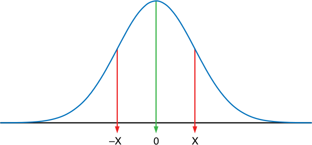
We obtain the values of N(x) by looking them up in a table. Below is an excerpt from a table of values of x. Suppose x = 0.75. Then we find the row containing the value 0.70 and move over to the column containing 0.05. The sum of the row value and the column value is the value of x. The corresponding probability is seen as the value 0.7734. Thus, N(0.75) = 0.7734. This means that the probability of obtaining a value of less than 0.75 in a normal distribution is 0.7734.

x	0	0.01	0.02	0.03	0.04	0.05	0.06	0.07	0.08	0.09
0.4	0.6554	0.6591	0.6628	0.6664	0.6700	0.6736	0.6772	0.6808	0.6844	0.6879
0.5	0.6915	0.6950	0.6985	0.7019	0.7054	0.7088	0.7123	0.7157	0.7190	0.7224
0.6	0.7257	0.7291	0.7324	0.7357	0.7389	0.7422	0.7454	0.7486	0.7517	0.7549
0.7	0.7580	0.7611	0.7642	0.7673	0.7704	0.7734	0.7764	0.7794	0.7823	0.7852
0.8	0.7881	0.7910	0.7939	0.7967	0.7995	0.8023	0.8051	0.8078	0.8106	0.8133
0.9	0.8159	0.8186	0.8212	0.8238	0.8264	0.8289	0.8315	0.8340	0.8365	0.8389
1.0	0.8413	0.8438	0.8461	0.8485	0.8508	0.8531	0.8554	0.8577	0.8599	0.8621
1.1	0.8643	0.8665	0.8686	0.8708	0.8729	0.8749	0.8770	0.8790	0.8810	0.8830

Alternatively (and somewhat easier) to looking up the value in a table we could have used a program like Excel to quickly compute the probability using the NORMSDIST function, so NORMSDIST(0.75) = 0.7734.

Now, suppose the value of x is negative. Observe in the figure above that the area to the left of-x is the same as the area to the right of +x. Therefore, if x is a negative number, N(x) is found as 1 – N(x). For example, let x = –0.75. We simply look up N(–x) = N[–(–0.75)] = N(0.75) = 0.7734. Then N(–0.75) = 1 – 0.7734 = 0.2266.

Let us now examine the various inputs required by the Black-Scholes model. We need to know where to get the inputs and how the option price changes when these inputs change.

3.     Inputs to the Black-Scholes Model

The Black-Scholes model has five inputs: the underlying price, the exercise price, the risk-tree rate, the time to expiration, and the volatility.¹

Call option prices should be higher the higher the underlying price, the longer the time to expiration, the higher the volatility, and the higher the risk-free rate. They should be lower the higher the exercise price. 

Put option prices should be higher the higher the exercise price and the higher the volatility. They should be lower the higher the underlying price and the higher the risk-free rate. As we saw in in our lesson on Fundamentals of Option Pricing, European put option prices can be either higher or lower the longer the time to expiration. American put option prices are always higher the longer the time to expiration, but the Black-Scholes model does not apply to American options.

These relationships apply to all European and American options and the Black-Scholes model is not required to understand these. Nonetheless, the Black-Scholes model provides an excellent opportunity to dig further into these relationships. We can calculate and draw connections like the ones above, which are known as option Greeks because they are frequently referred to with Greek names. Let us now examine each of the inputs as well as the various option Greeks.

3.1      The Underlying Price: Delta and Gamma

The price of the underlying is generally one of the easiest sources of input information. Suffice to say that if an investor cannot obtain the price of the underlying, then he should not even be considering the option. The price should generally be obtained as a quote or trade price from a liquid, open market. The relationship between the option price and the underlying price is known as the option delta. In fact, the delta can be obtained approximately from the Black-Scholes formula as the value of N(d₁) for calls and N(d₁) – 1 for puts. More formally, the delta is defined as

Delta = Change in option price / Change in underlying price

The above definition for delta is exact; the use of N(d₁) for calls and N(d₁) – 1 for puts is approximate. Later in this section, we shall see why N(d₁) and N(d₂) are approximations and when they are good or bad approximations.

Let us consider the example we previously worked with, where S = 100, X = 100, r= 0.030, T = 0.50, and σ = 0.25. Using Excel to obtain a more precise Black-Scholes answer, we get a call option price of 7.7603 and a put option price of 6.2715. N(d₁), the call delta, is 0.5688, so the put delta is 0.5688 – 1 = –0.4312. Given that Delta = (Change in option price/Change in underlying price), we should expect that:

Change in option price = Delta * Change in underlying price.

Therefore, for a $1 change in the price of the underlying, we should expect:

Change in call option price = 0.5688 * 1 = 0.5688

Change in put option price = –0.4312* 1 = –0.4312

This calculation would mean that:

Approximate new call option price = 7.7603 + 0.5688 = 8.3290

Approximate new put option price = 6.2715 – 0.4312 = 5.8402

To test the accuracy of this approximation, we let the underlying price move up $1 to $101 and re-insert these values into the Black-Scholes model.

We would then obtain:

Actual new call option price = 8.3401

Actual new put option price = 5.8513

The delta approximation is fairly good, but not perfect.

Delta is a significant risk indicator. The delta expresses the sensitivity of the option price to changes in the underlying price. Traders, particularly option dealers, utilize delta to build hedges to balance the risk they take by buying and selling options. Assume we’re a dealer proposing to sell the call option we’ve been dealing with previously. A customer buys 1,000 options for 7.7603 per option contract. We are now short 1,000 call option contracts, which exposes us to significant risk if the underlying rises. To hedge this risk, we must purchase a fixed number of units of the underlying. We have previously shown that the delta is 0.5688, implying that we would purchase 569 units of the underlying at 100. Assume for the time being that the delta indicates the exact movement in the option for a movement in the underlying. Assume the underlying rises by $1:

Change in value of 569 long units of the underlying: 569 * 1 = 569

Change in value of 1,000 short options: 1,000 * 1 * 0.5688 = 569

These numbers offset because we are long the underlying and short the options. At this point, however, the delta has changed. If we recalculate it, we would find it to be 0.5903.  This would require us to have 590 units of the underlying, which would necessitate the purchase of an extra 21 units. To achieve this, we would have to borrow money. In other situations, we would need to sell units of the underlying, in which case the proceeds would be invested in the risk-free asset.

Consider how changes in the underlying price affect the delta. Even if the underlying price does not change, the delta will fluctuate as the option approaches expiration. For a call, the delta will rise toward 1.0 as the underlying price rises and fall toward 0.0 as the underlying price falls. The delta for a put will drop toward –1.0 as the underlying price falls and increase toward 0.0 as the underlying price rises. If the underlying price does not change, the call delta will move toward 1.0 if the call is in-the-money or 0.0 if the call is out-of-the-money as the call approaches expiry. As the expiration date approaches, a put delta will move toward –1.0 if the put is in-the-money and toward 0.0 if the put is out-of-the-money.

Delta hedging is a dynamic process since the delta is continually changing. In fact, delta hedging is often known as dynamic hedging. In principle, the delta changes continually, thus the hedge should be changed continually, but in practice, continuous adjustment is not practical. When the hedge is not regularly modified, we accept the prospect of much larger price changes in the underlying. Let us see what happens in that case.

Using our previous example, we assume an increase in the underlying price of $10 to $110. Then the call price should change by 0.5688 * 10 = 5.688, and the put option price should change by –0.4312 * 10 = –4.312. Thus, the approximate prices would be:

Approximate new call option price = 7.7603 + 5.688 = 13.4479

Approximate new put option price = 6.2715 – 4.312 = 1.9591

The actual prices are obtained by recalculating the option values using the Black-Scholes model with an underlying price of 100. Using Excel, we find that these prices are:

Actual new call option price = 14.4670

Actual new put option price = 2.9782

The approximations based on delta are not very accurate. In general, the larger the move in the underlying. the worse the approximation. This will make delta hedging less effective.

The below Exhibit shows the relationship between the option price and the underlying price. Notice the curvature in the relationship between the option price and the underlying price. Call option values definitely increase the greater the underlying value, and put option values definitely decrease. But the amount of change is not the same in each direction. N(d₁) measures the slope of this line at a given point. As such, it measures only the slope for a very small change in the underlying. When the underlying changes by more than a very small amount, the curvature of the line comes into play and distorts the relationship between the option price and underlying price that is explained by the delta. The problem here is much like the relationship between a bond price and its yield. This first-order relationship between a bond price and its yield is called the duration; therefore, duration is similar to delta.

Exhibit: The Relationship between Option Price and Underlying Price X = 100, r^c = 0.03, T = 0.50, σ = 0.25

Call	Put

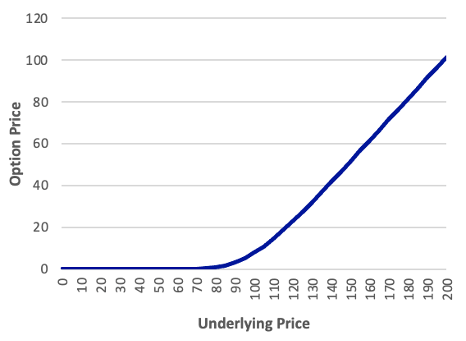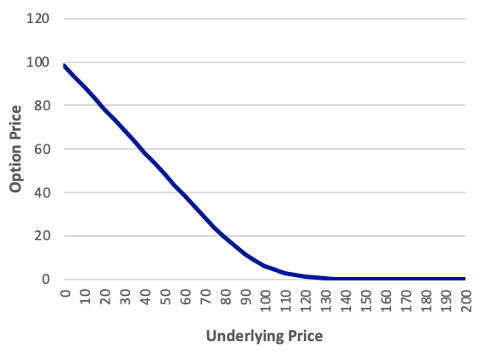In the field of fixed income, the curvature or second-order impact is referred to as convexity. This impact is known as gamma in the options world. Gamma is a numerical measure of the delta’s sensitivity to changes in the underlying, or how much the delta changes. When gamma is big, the delta changes rapidly and cannot offer an accurate estimate of how much the option moves for each unit of movement in the underlying. We will not be concerned with measuring and utilizing gamma, but we should know a few facts about gamma and, by extension, delta behavior.

Gamma is larger when there is more uncertainty about whether the option will expire in- or out-of-the-money. This means that gamma will tend to be large when the option is at the money and close to expiration. As a result, delta will be a poor approximation for the option’s price sensitivity when it is at-the-money and near to expiration. As a result, a delta hedge will perform badly. When the gamma is large, we may need to apply a gamma-based hedge, which would require that we add a position in another option to the delta-hedge position of the underlying and the option. We will not discuss this sophisticated subject further here.

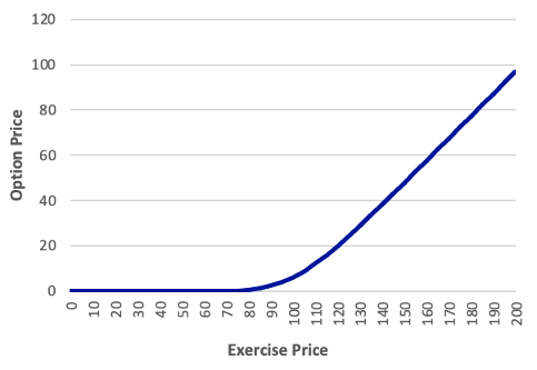
3.2      The Exercise Price

The exercise price is simple to determine. It is defined in the option contract and remains constant. As a result, it is pointless to discuss what occurs when the exercise price changes, but we may discuss how the option price would fluctuate if we chose an option with a different exercise price. As previously demonstrated, the greater the exercise price, the lower the call option price and the higher the put option price. The Exhibit below confirms this relationship.

Exhibit: The Relationship between Option Price and Exercise Price S = 100, r^c = 0.03, T = 0.50, σ = 0.25

Call	Put

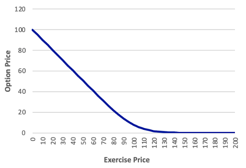3.3      The Risk-Free Rate: Rho

The risk-free rate is the continuously compounded rate on the risk-free security whose maturity corresponds to the option’s life. We have used the risk-free rate in previous readings; sometimes we have used the discrete version and sometimes the continuous version. As we have noted, the continuously compounded risk-free rate is the natural log of 1 plus the discrete risk-free rate.

For example, suppose the discrete risk-free rate quoted in annual terms is 3.0 percent. Then the continuous rate is:

r^c = ln(1 + r) = ln (1.03) = 0.0296

Let us recall the difference in these two specifications. Suppose we want to find the present value ot $1 in six months using both the discrete and continuous risk-free rates:

Present value using discrete rate = 1 / (1 + r)^T = 1 / (1.03)^0.5 = 0.9853

Present value using continuous rate = e^-rcT = e^-0.0296(0.5) = 0.9853  

Clearly, either specification will suffice. Because of how it uses the risk-free rate in the calculation of d₁however, the Black-Scholes model requires the continuous risk-free rate.

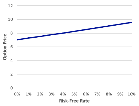
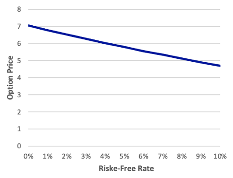
The sensitivity of the option price to the risk-free rate is called the rho. We shall not concern ourselves with the calculation of rho. Technically, the Black-Scholes model implies a constant risk-free rate, therefore talking about the risk-free rate increasing during the life of the option has less meaning. We may, however, investigate how the option price would change if the current rate changed were different. This impact is depicted in the exhibit below. Take note of how little variation there is in the option price across a wide variety of risk-free rates. The price of a European option on an asset is, in fact, not highly sensitive to the risk-free rate.²

Exhibit: The Relationship between Option Price and Risk-Free Rate S = 100, X = 100, T = 0.50, σ = 0.25

Call	Put

3.4      Time to Expiration: Theta

The time until expiry is a simple input to calculate. The contract specifies a defined expiration date for the option. We simply divide the number of days till expiry by 365.

Obviously, the time remaining in an option’s life moves constantly towards zero. Even if the underlying price is constant, the option price will still change. American options have both an intrinsic value and a time value. All of the pricing for European options may be interpreted as time value. In any scenario, time value is determined by the moneyness of the option, its time to expiry, and its volatility. The bigger the uncertainty, the larger the time value. As the option’s expiration date approaches, the option price advances toward the option’s payoff value at expiry, a process known as time value decay. The option’s theta is the pace at which the time value decays. We won’t worry about determining the exact amount of theta, but keep in mind that if the option price falls over time, the theta will be negative. The time value decay for our example option is depicted in the exhibit below.

Exhibit: The Relationship between Option Price and Time to Expiration S = 100, X = 100, r^c = 0.03, σ = 0.25

Call	Put

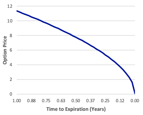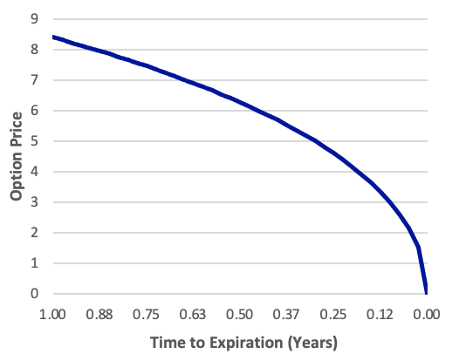We observe that the call and put values both decline as the time to expiry decreases. As previously stated, European put options do not always do this. In certain situations, the value of European put options increases as the time to expiry reduces, like in the case of a positive theta, but this is not the case with our put.³

Most of the time, option prices are higher the longer the time to expiration. For European puts, however, some exceptions exist.

3.5      Volatility: Vega

Volatility is defined as the standard deviation of the stock’s continuously compounded return. Volatility is an incredibly essential component in option value. It is the only variable that cannot be simply and directly retrieved from another source. Furthermore, as we show below, option prices are extremely sensitive to volatility.

The link between option pricing and volatility is known as the vega, which, though being regarded an option Greek, is not a Greek word. We will not worry ourselves with the precise computation of the vega, but we will note that the vega is positive for both calls and puts, implying that if volatility rises, so will the prices of both call and put options. Furthermore, the vega increases as the option gets closer to being at-the-money.

In the problem we previously worked with (S₀ = 100, X = 100, r = 0.03, T = 0.50), at a volatility of 0.25, the option price was 7.76. Suppose we erroneously use a volatility of 0.30. Then the call price would be 9.15. An error of this magnitude in volatility would be easy to make, especially for a variable that is not directly observable. However, the result is a very large error in the option price.

The below Exhibit displays the relationship between the option price and the volatility. Note that this relationship is nearly linear and that the option price varies over a very wide range, although this near-linearity is not the case for all options.

Exhibit: The Relationship between Option Price and Volatility S = 100, X = 100, r^c = 0.03, T = 0.50

Call	Put

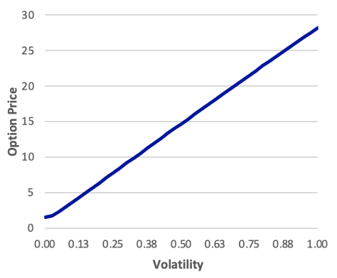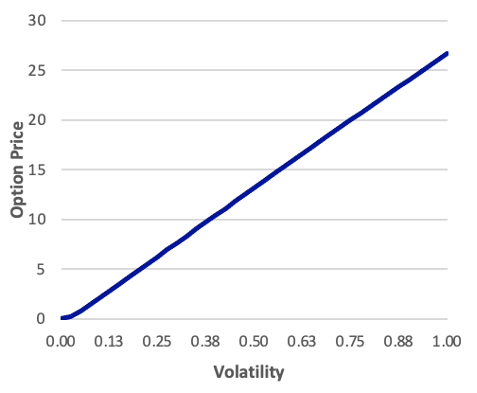4.     The Effect of Cash Flows on the Underlying

Cash flows on the underlying also have an impact on the pricing of options and other derivative instruments. We saw previously in our reading about option boundary conditions and put-call parity that we subtract the present value of the dividends from the underlying price and use this adjusted price to establish the boundary conditions or to price the options using put-call parity. We do the same using the Black-Scholes model. Specifically, we introduced the expression PV(CF, 0, T) for the present value of the cash flows on the underlying over the life of the option. So, we simply use S₀ – PV(CF, 0, T) in the Black-Scholes model instead of S₀.

Previously we also used continuous compounding to express the cash flows. For stocks, we used a continuously compounded dividend yield; for currencies, we used a continuously compounded interest rate. In the case of stocks, we let δ^c represent the continuously compounded dividend rate. Then we substituted S₀e^–δcT for S₀ in the Black-Scholes formula. For a foreign currency, we let S₀ represent the exchange rate, which we discount using r^fc, the continuously compounded foreign risk-free rate. Let us work an example involving a foreign currency option.

Let the exchange rate of U.S. dollars for euros be $1.10. The continuously compounded U.S. risk-free rate, which in this example is r, is 3.0 percent. The continuously compounded euro risk-free rate, r^fc, is 2.0 percent. A call option expires in 145 days (T= 145/365 = 0.3973) and has an exercise price of $1.15. The volatility of the continuously compounded exchange rate is 0.075.

The first thing we do is obtain the adjusted price of the underlying: 1.10e^{–0.02(0.3973)} = 1.0913. We then use this value as S₀ in the formula d₁ and d₂:

d₁ = (ln(1.0913/1.15) + [0.03 + 0.075²/2] * 0.3973) / (0.075 * 0.3973^0.5) = –0.8326

d₂ = –0.8326– 0.075 * 0.3973^0.5 = –0.8799

Using the normal probability distribution, we find that   

N(d₁) = N(–0.8326) = 1 – 0.7975 = 0.2025

N(d₂) = N(–0.8799) = 1 – 0.8105 = 0.1895

In discounting the exercise rate to evaluate the second term in the Black-Scholes expression, we use the domestic (here, U.S.) continuously compounded risk-free rate. The call option price would thus be

c = 1.0913 * 0.2025 – 1.15e^{–0.03(0.3973)} * 0.1895 = 0.00565

Therefore, this call option on an asset worth $1.10 would cost $0.00565.

5.     The Critical Role of Volatility

As we have previously highlighted, volatility is an extremely important variable in the pricing of options. In fact, with the possible exception of the cash flows on the underlying, it is the only variable that cannot be directly observed and easily obtained. It is, after all, the volatility over the life of the option; therefore, it is not past or current volatility but rather the future volatility. Differences in opinion on option prices nearly always result from differences of opinion about volatility. But how does one obtain a number for the future volatility?

5.1      Historical Volatility

Past volatility is the most reasonable place to look for an estimate of future volatility. When the underlying is a publicly traded asset, we can generally collect some data from the recent past and estimate the standard deviation of the continuously compounded return.

The Exhibit below depicts this approach for a sample of 12 monthly prices for a specific company. We convert these prices to returns, then to continuously compounded returns, calculate the variance of the series of continuously compounded returns, and finally the standard deviation.

Because the data in this case are monthly returns, we must annualize the variance by multiplying it by 12. The square root is then used to get the historical estimate of the yearly standard deviation or volatility.

The historical volatility estimate is based only on what has occurred in the past. We need to utilize a lot of prices to achieve the best estimate, but it implies going back further in time. The farther we go back in time, the less current the data becomes, and the less trustworthy our estimate of volatility becomes. We now look at a method for generating a more recent estimate of volatility, but one that raises questions as well as answers them.

Exhibit: Estimating Historical Volatility

Month	Price	Return	Log Return	(Log Return – Avg.)2
0	100
1	103	0.030000	0.029559	0.000572
2	97	-0.058252	-0.060018	0.004311
3	90	-0.072165	-0.074901	0.006487
4	93	0.03333	0.032790	0.000737
5	87	-0.064516	-0.066691	0.005232
6	100	0.149425	0.139262	0.017855
7	96	-0.04000	-0.040822	0.002159
8	105	0.093750	0.089612	0.007052
9	110	0.047619	0.046520	0.001671
10	105	-0.045455	-0.046520	0.002720
11	103	-0.019048	-0.019231	0.000618
12	107	0.038835	0.038100	0.001054
		Sum	0.067659	0.050468
		Average	0.005638

5.2      Implied Volatility

In a market in which options are traded actively, we can reasonably assume that the market price of the option is an accurate reflection of its true value. Thus, by making the Black-Scholes price equal to the market price, we may deduce volatility backwards. This approach allows us to determine the volatility used by option traders to price the option. This is referred to as implied volatility.

Unfortunately, calculating implied volatility is not an easy task. For volatility, we cannot simply solve the Black-Scholes equation. It is a complicated function in which the volatility appears a number of times, in some cases as σ².

The variance is estimated as follows:

σ² = Σ(R_i^c – R^c)2 / (N – 1)

Where R_i^c is the continuously compounded return for observation i (shown above in the fourth column and calculated as In(1 + R_i), where i goes from 1 to 12) and R_i is the ith return, R^c is the average return over the entire sample, and N is the number of observations in the sample (here, N = 12). Then:

σ² = 0.05047 / 11 = 0.004588

Because this sample consists of monthly returns, to obtain the annual variance, we must multiply this number by 12 (or 52 for weekly, or 250—the approximate number of trading days in a year-for daily). Thus:

σ = 12 * 0.004588 = 0.05506

The annual standard deviation or volatility is, therefore:

σ = 0.05506^0.5 = 0.2346

So the historical volatility estimate is 23.46 percent.

There are some mathematical techniques that speed up the estimation of the implied volatility. Here, however, we shall look at only the most basic method: trial and error.

Recall the option we have been working with. The underlying price is 100 the exercise price is 100, the risk-free rate is 3.0 percent, and the time to expiration is 0.50. In our previous examples, the volatility was 0.25. Using these values in the Black-Scholes model, we obtained a call option price of 7.7603. Suppose we observe the option selling in the market for 8.50. What volatility would produce this price?

We have already calculated a price of 7.7603 at a volatility of 0.25. Because the call price varies directly with the volatility, we know that it would take a volatility greater than 0.25 to produce a price higher than 7.7603. We do not know how much higher, so we should just take a guess. Let us try a volatility of 0.30. Using the Black-Scholes formula with a volatility of 0.30, we obtain a price of 9.1494. This is too high, so we try a lower volatility. We keep doing this in the following manner:

Volatility	Black-Scholes Price
0.25	7.7603
0.30	9.1494
0.29	8.8716
0.28	8.5939
0.27	8.3160

So, we now know that the correct volatility is between 0.27 and 0.28, closer to 0.28. When calculating implied volatility, we must decide either how close to the option price we want to be or how many significant digits we want in the implied volatility. If we use four significant digits in the implied volatility, a value of 0.276622 results in an option price of 8.5000.

As a result, if the option is selling for about 8.50, we say that the market is pricing it at a volatility of 0.2766. This figure indicates the market’s best assessment of the underlying asset’s true volatility; it is a more recent source of volatility information than historical volatility.

Unfortunately, the argument has a circularity. If the Black-Scholes model is used to assess whether an option is overpriced or underpriced, the technique for calculating implied volatility presupposes that the market accurately values the option. The implied volatility can only be used to identify mispriced options if it is interpreted as either too high or too low, which requires an assessment of true volatility. Nonetheless, the implied volatility is a source of valuable information in regards to the uncertainty in the underlying, and option traders use it frequently.

---

---

1. Later we shall add one more input, cashflows on the underlying.[↩]
2. Except when the underlying is an interest rate. In this specific case there is a strong relationship between the option price and interest rates.[↩]
3. Positive put thetas tend to Occur when the put is deep in-the-money, the volatility is low, the interest rate is high, and the time to expiration is low.[↩]