The binomial model is the technique we’re introducing here. The term “binomial” refers to the fact that there are just two possibilities. In other words, we only allow the underlying price to shift to one of two new values. As previously stated, this framework oversimplifies things; nonetheless, the model may eventually be expanded to include all conceivable prices. Furthermore, the structure of this model is referred to as discrete time, which indicates that time flows in separate increments. This is like looking at a calendar and just noticing the months, weeks, or days. We know that time travels quicker than one day at a time, even at its shortest interval. It moves in hours, minutes, seconds, and even fractions of seconds, and fractions of fractions of seconds. When we talk about time moving in minuscule increments, we are referring to continuous time. We’ll examine how the discrete time model may be transformed into a continuous time model.

The more advanced continuous time model (Black-Scholes-Merton) is presented in our next lesson, however the binomial model has the benefit of allowing us to price American options. Furthermore, the binomial model is a basic model that requires very little mathematics. As a result, it is worth studying in its own right.

This reading is part of our introductory options course. Please check out the full overview of lessons here.

1.     The One-Period Binomial Model

We start off by having only one binomial period. This means that the underlying price starts off at a given level, then moves forward to a new price, at which time the option expires. Here we need to change our notation slightly from what we have been using previously. We let S be the current underlying price. One period later, it can move up to S⁺ or down to S^–. Note that we are removing the time subscript, because it will not be necessary here. We let X be the exercise price of the option and r be the one period risk-free rate. The option is European style.

1.1      The Model

We start with a call option. If the underlying goes up to S⁺, the call option will be worth c⁺. If the underlying goes down to S^–, the option will be worth c^–. We know that when the option expires, its value will be the intrinsic value. Thus:

c⁺ = Max (0, S⁺ – X)

c^– = Max (0, S^– – X)

Exhibit: One-Period Binomial Model

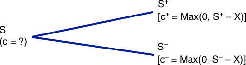
This scenario is depicted in the preceding Exhibit using a diagram known as a binomial tree. Note how we indicate that the current option price, c, is unknown. Let us now define how the underlying moves. We designate a factor u as the underlying’s up motion and a factor d as the underlying’s down move:

u = S⁺ / S

d = S^– / S

u and d represent 1 plus the rate of return if the underlying goes up and down, respectively. Thus, S⁺ = Su and S^– = Sd. To avoid an obvious arbitrage opportunity, we require that:

d < 1 + r < u

We’re now ready to figure out how to price the option. Except for the current option price, we assume we have all of the required information.  Furthermore, we are not sure which way the underlying price will move. To start, we create an arbitrage portfolio comprised of one short call option. Let us now buy an unspecified number of underlying units. Let that number be n. Although we do not yet know the value of n, we can figure it out quickly. This is referred to as a hedging portfolio. In fact, n is sometimes referred to as the hedge ratio. Its current value is H, where:

H = nS – c

This specification reflects the fact that we own n units of the underlying worth S and we are short one call.¹ One period later, this portfolio value will move to either H⁺ or H^–:

H⁺ = nS⁺ – c⁺

H^– = nS^– – c^–

Because we can choose the value of n, let us do so by setting H⁺ equal to H^–. This specification means that the portfolio value will remain constant regardless of how the underlying fluctuates. As a result, the portfolio will be hedged. We do this by setting:

H⁺ = H^–, which means that:

nS⁺ – c⁺ = nS^– – c^–

We then solve for n to obtain:

n = (c⁺ – c^–) / (S⁺ – S^–)

We can simply set n using this method because the numbers on the right-hand side are known. The portfolio will be hedged if we do so. A hedged portfolio should grow in value at the risk-free rate.

H⁺ = H * (1 + r), or

H^– = H * (1 + r)

As we know that H⁺ = nS⁺ – c⁺, H^– = nS^– – c^–, and H = nS – c. We know the values of n, S⁺, S^–, c⁺ and c^–, as well as r. We can substitute and solve either of the above for c to obtain:

c = (πc⁺ + (1 – π)c^–) / (1 + r)

where:

π = (1 + r – d) / (u – d)

We see that the call price today, c, is a weighted average of the next two possible call prices, c⁺ and c^–. The weights are π and 1 – π. This weighted average is then discounted back one period at the risk-free rate. 

It might appear that π and 1 – π are probabilities of up and down movements, but they are not. In fact, the probabilities of up and down movements are not required. However, it is important to emphasize that π and 1 – π are the probability that would occur if investors were risk averse. Assets are valued by risk-neutral investors by calculating the projected future value and discounting it at the risk-free rate. Because we are discounting at the risk-free rate, it should be obvious that π and 1 – π would be the probability if the investor were risk averse. In fact, we shall refer to them as risk-neutral probabilities and the process of valuing an option is often called risk-neutral valuation.²

1.2      One-Period Binomial Example

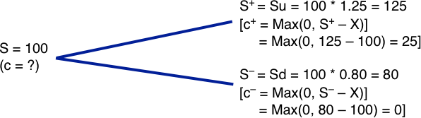
Suppose the underlying is a non-dividend-paying stock currently valued at 100. It can either increase by 25 percent or decline by 20 percent. Thus, u = 1.25 and d = 0.80.

S⁺ = Su = 100 * 1.25 = 125

S^– = Sd = 100 * 0.80 = 80

Assume that the call option has an exercise price of 100 and the risk-free rate is 3 percent. Thus, the option values one period later will be:

c⁺ = Max (0, S⁺ – X) = Max(0, 125 – 100) = 25

c^– = Max (0, S^– – X) = Max(0, 80 – 100) = 0

The below Exhibit depicts this situation.

Exhibit: One-Period Binomial Example

First we calculate π:

π = (1 + r – d) / (u – d) = (1.03 – 0.80) / (1.25 – 0.80) = 0.51

Hence 1 – π = 0.49. Now, we can directly calculate the option price:

c = (0.51 * 25 + 0.49 * 0) / (1.03) = 12.38

Thus, the option should sell for 12.38.

1.3      One-Period Binomial Arbitrage Opportunity

Assume the option sells for 14. If the option should be selling for 12.38 but instead sells for 14, it is overpriced—a clear instance of price not equaling value. Investors would take advantage of this opportunity by selling the option and purchasing the underlying. The value n represents the number of units of the underlying acquired for each option sold:

n = (c⁺ – c^–) / (S⁺ – S^–) = (25 – 0) / (125 – 80) = 0.556

Thus, for every option sold, we would buy 0.556 units of the underlying. Suppose we sell 1,000 calls and buy 556 units of the underlying. Doing so would require an initial outlay of H = 556 * 100 – 1,000 * 14 = 41,600. One period later, portfolio value will be either:

H⁺ = nS⁺ – c⁺ = 556 * 125 – 1,000 * 25 = 44,500

H^– = nS^– – c^– = 556 * 80 – 1,000 * 0 = 44,480

The two values are not exactly the same, but the difference is due only to rounding the hedge ratio, n. We shall use the 44,500 value. If we invest 41,600 and end up with 44,500 the return is:

44,500 / 41,600 – 1 = 0.0697

That is a risk-free return of 6.97 percent in contrast to the actual risk-free rate of 3 percent. Thus we could borrow $41,600 at 3 percent to finance the initial net cash outflow, capturing a risk-free profit of (0.0697 – 0.03) * 41,600 = 1,651 without investing any money. Other investors will recognize this opportunity and begin selling the option, which will drive down its price. When the option sells for $12.38, the initial outlay would be H= 556 * 100 – 1,000 * 12.38) = 43,220. The payoffs at expiration would still be 44,500. This transaction would generate a return of:

44,500 / 43,220 – 1 = 0.030

Thus, when the option is trading at the price given by the model, a hedge portfolio would earn the risk-free rate, which is appropriate because the portfolio would be risk free.

If the option price is less than 12.38, investors would buy the option and sell short the underlying, generating cash up front. At the end of the term, the investor would have to pay back less than 3%. This transaction would be carried out by all investors, creating demand for the option and pushing its price back up to 12.38.

2.     The Two-Period Binomial Model

In the preceding example, the underlying movement was portrayed during a single period, and there were just two outcomes. We can expand the model to get more realistic results with more than two outcomes. The below Exhibit shows how to do so with a two-period binomial tree.

Exhibit: Two-Period Binomial Model

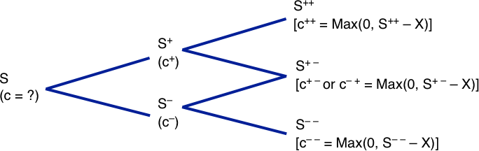
In the first period, we let the underlying price move from S to S⁺ or S^– in the manner we did in the one-period model. That is, if u is the up factor and d is the down factor:

S⁺ = Su

S^– = Sd

Then, with the underlying at S⁺ after one period, it can either move up to S⁺⁺ or down to S^+–. Thus:

S⁺⁺ = S⁺u

S^+– = S⁺d

If the underlying is at S^– after one period, it can either move up to S^–+ or down to S^{– –}

S^–+ = S^–u

S^{– –} = S^–d

We now have three unique final outcomes instead of two. In fact, we have four final outcomes, but S^+– is the same as S^–+. We can relate the three final outcomes to the starting price in the following manner:

S⁺⁺ = S⁺u = Suu = Su²

S^+– (or S^–+) = S⁺d (or S^–u) = Sud (or Sdu)

S^{– –} = S^–d = Sdd = Sd²

Now we move forward to the end of the first period. Suppose we are at the point where the underlying price is S⁺. Note that now we are back into the one-period model we previously developed. There is one period to go and two outcomes. The call price is c⁺ and can go up to c⁺⁺ or down to c^+–. Using what we know from the one-period model, the call price must be:

c⁺ = (πc⁺⁺ + (1 – π)c^+–) / (1 + r)

Again, we see that the call price is a weighted average of the next two possible call prices discounted back one period. If the underlying price is at S^–, the call price would be:

c^– = (πc^–+ + (1 – π)c^{– –}) / (1 + r)

In both cases the formula for π remains:

π = (1 + r – d) / (u – d)

Again, the call price is a weighted average of the next two possible call prices, discounted back to the present. Aside from knowing the formula for π, the call price formula is simple and intuitive. It is the average of the following two possibilities, weighted by the risk-neutral probability, discounted to the present.³

Recall that the hedge ratio, n, was given as the difference in the next two call prices divided by the difference in the next two underlying prices. This will hold true in all cases throughout the binomial tree. Hence, we have different hedge ratios at each time point:

n = (c⁺ – c^–) / (S⁺ – S^–)

n = (c⁺⁺ – c^+–) / (S⁺⁺ – S^+–)

n = (c^–+ – c^{– –}) / (S^–+ – S^{– –})

2.1      Two-Period Binomial Example

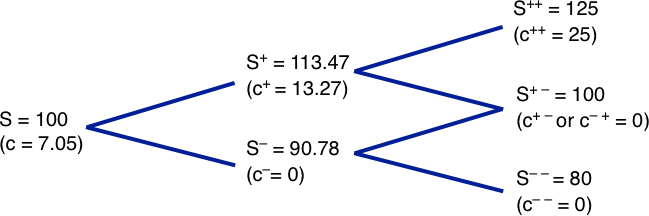
We can continue with the previous scenario in which the underlying increases by 25 percent or decreases by 20 percent. Let us, however, change the example somewhat. Assume the underlying increases by 11.8 percent or decreases by 10.56 percent, and we increase the number of periods to two. The up factor is thus 1.118, while the down factor is 1 – 0.1056 = 0.8944. If the underlying goes up for two consecutive periods, it rises by a factor of 1.118 * 1.118 = 1.25 (25 percent). If it goes down in both periods, it falls by a factor of 0.8944 * 0.8944 = 0.80 (20 percent). This specification makes the highest and lowest prices unchanged. Let the risk-free rate be 1.489 percent per period. Then π becomes (1.01489 – 0.8944) / (1.118 – 0.8944) = 0.5389. The underlying prices at expiration will be:

S⁺⁺ = Su² = 100 * 1.118 * 1.118 = 125

S^+– = Sud = 100 *1.118 * 0.8944 = 100

S^{– –} = Sd² = 100 * 0.8944 * 0.8944 = 80

When the options expire, they will be worth:

c⁺⁺ = Max (0, S⁺⁺ – 100) = Max(0, 125 – 100) = 25

c^+– = Max (0, S^+– – 100) = Max(0, 100 – 100) = 0

c^{– –} = Max (0, S^{– –} – 100) = Max(0, 80 – 100) = 0

The option values after one period are, therefore:

c⁺ = (πc⁺⁺ + (1 – π)c^+–) / (1 + r) = (0.5389 * 25 + 0.4611 * 0) / (1.01489) = 13.27

c^– = (πc^–+ + (1 – π)c^{– –}) / (1 + r) = (0.5389 * 0 + 0.4611 * 0) / (1.01489) = 0

So, the option price today is:

c⁺ = (πc⁺ + (1 – π)c^–) / (1 + r) = (0.5389 * 13.27 + 0.4611 * 0) / (1.01489) = 7.05

These results are summarized in the Exhibit below.

Exhibit: Two-Period Binomial Example

We will not illustrate an arbitrage opportunity since doing so would necessitate a lengthy and thorough example that would be excessive for our purposes. Suffice it to say, if the option is mispriced, one can build a hedged portfolio that will generate a return greater than the risk-free rate.

3.     Binomial Put Option Pricing

In the previous Section, the option was a call. Making the option a put is a straightforward process. We could go back through the entire example, changing all c’s to p’s and using the formulas for the payoff values of a put instead of a call. We should note, however, that if the same formula used for a call is used to calculate the hedge ratio, the minus sign should be ignored as it would suggest being long the stock (put) and short the put (stock) when the hedge portfolio should actually be long both instruments or short both instruments. The put moves opposite to the stock in the first place: hence, long or short positions in both instruments are appropriate.

4.     American Options

The binomial model is also well suited to dealing with American style options. At any point in the binomial tree, we can determine whether the calculated value of the option is exceeded by its value if exercised early. If this is the case, the calculated value is replaced with the exercise value.

5.     Extending the Binomial Model

In the examples in this reading, we are dividing the life of an option into a certain number of periods. Assume we’re pricing a one-year contract. If we just utilize one binomial period, we will only obtain two prices for the underlying, which is unlikely to yield a satisfactory outcome. If we utilize two binomial periods, the underlying will have three prices at expiry. This outcome would most likely be better, but still not very good. However, as the number of periods increases, the outcome should become more accurate. In fact, in the limiting case, we are likely to get a very good result. By increasing the number of periods, we are moving from discrete time to continuous time.

Consider the following example of a one-period binomial model for a six month option. The asset is priced at 100. It can increase by 19.34 percent or decrease by 16.20 percent, so u = 1.1934 and d = 1 – 0.1620 = 0.8380. The risk-free rate is 3 percent. A call option has an exercise price of 100 and expires in six months. Using a one-period binomial model would obtain an option price of 9.4947. The Exhibit below demonstrates the results obtained by dividing the six-month option life into an increasing number of shorter and shorter periods. However, the method by which we fit the binomial tree is not arbitrary since we must change the values of u, d, and the risk-free rate so that the underlying price move is reasonable over the life of the option. The volatility is connected to how we change u and d. In fact, we don’t need to worry about how to change any of these variables; all we need to do is notice that our binomial option price looks to be converging to a value of approximately 7.76.

ln the same way a sequence of rapidly taken still photographs converges to what appears to be a continuous sequence of a subject’s movements, the binomial model converges to a continuous-time model, the subject of our next lesson.

Exhibit: Binomial Option Prices for Different Numbers of Time Periods

Number of Time Periods	Option Price
1	9.4947
2	6.9621
5	8.1104
10	7.5873
25	7.8294
50	7.7253
100	7.7427
500	7.7567
1,000	7.7585

---

---

1. This statement states that if the underlying price rises, it must do so at a rate greater than the risk-free rate. If it falls, it must fall at a lower rate than the risk-tree rate. If the underlying consistently outperforms the risk-free rate, it would be conceivable to acquire the underlying, finance it with risk-free borrowing, and be certain of getting a higher return from the underlying than the cost of borrowing. This would allow you to produce an infinite quantity of money. If the underlying constantly performs worse than the risk-free rate, the risk-free asset can be purchased and financed by shorting the underlying. This would also allow you to earn an infinite quantity of money. As a result, neither the risky underlying asset nor the risk-free asset can dominate or be dominated by the risk-free asset. Think of this specification as a plus sign indicating assets and a minus sign indicating liabilities.[↩]
2. It may be useful to contrast risk neutrality with risk aversion, which is common in almost all individuals. Risk neutral individuals evaluate an asset, such as an option or stock, by discounting the projected value at the risk-free rate. Risk averse people discount the projected value at a higher rate, one that includes the risk-free rate plus a risk premium. We do not assume that individuals are risk neutral when valuing options, but the fact that options may be priced by calculating the anticipated value, applying these particular probabilities, and discounting at the risk-free rate gives the impression that investors are risk neutral. We stress the word “appearance” since such an assumption is not formed. The words “risk neutral probability” and “risk neutral valuation” are commonly used in options valuation, although they give a misleading impression of the assumptions underlying the process.[↩]
3. It is also possible to represent the price today as a weighted average of the three final option prices discounted two periods, so eliminating the intermediate step of determining c+ and c–; however, there is little value in doing so, and this technique is slightly more technical.[↩]